Cross Tabulation
We have carried out cross tabulation for several
variables of our questionnaires. Firstly, we have cross tabulated household
income with tuition class. Based on the results (Appendix
1), 58.33% of our low-income respondents will send their children for
attending tuition class whereas the remaining 41.67% will not send their
children to tuition class.


In order to further study the number of tuition classes being attended by their children, we have carried another cross tabulation between household income and sum of tuition classes attended. The types of tuition classes include school-related, language, drawing, music and dancing. By referring to the results (Appendix 2), half of the low-income respondents do send their children to attend at least one tuition class. It is followed by 5.95% of them sending their children to attend two tuition classes and 2.38% of their children are attending three tuition classes. There are 41.67% of the children do not attending any tuition classes and this figure have been mentioned in the above.


Besides that, we have also carried
out cross tabulation for the level of education that the parents expect their
children to achieve based on their household income. Based on the results
obtained (Appendix 3), 21.43% of the respondents
expect their children to study till SPM level only and 17.86% of them would
expect their children to attain A-level or Diploma level of education. On the
other hand, 42.86% of the low-income respondents expect their children to
attain Degree level of education followed by Master with 13.1% and PHD with
4.76%.
Moreover, cross tabulation between
the household income and saving for children’s education have also been done.
By referring to the results (Appendix 4), more
than half of the low-income respondents which are 51.19% do not save for their
children’s education. The remaining 48.81% do save money for their children’s
education.
We have also analysed the monthly saving amount of those who do save
for children’s education (Appendix 5). Based on
the results, 27.38% of the respondents save RM 100 and below; 10.71% save RM
101 to RM 200; and 3.57% save RM 201 to RM 300, RM 301 – RM 400 and RM 401 and
above respectively.
Additionally, we have also cross
tabulated the household income and the main reason that will affect parents’
decision to send their children to further their study. As referred to the
results (Appendix 6), 14.29% of the low-income
respondents would take children’s ability into consideration; relatives’
influence, 5.95%; children’s interest, 28.57%; financial, 46.43% and other
reason, 4.76%.
Linear Regression
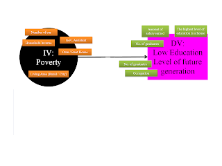
We have also conducted linear regression for
household income (IV) and sum of tuition classes (DV). In this case, household
income represents the independent variable and sum of tuition classes
represents dependent variable. Based on the ANOVA table (Appendix 7), the value of F statistic which is 5.084 is the
regression mean square divided by the residual mean square which is 2.100/0.413.
The significant value of the F statistic is 0.026, which is smaller than the
standard value, 0.05. Therefore, we can conclude that the independent variable,
which is household income do explain the variation in the dependent variable
which is tuition class.


Besides that, based on the model summary table (Appendix7),
the value of R is 0.222 and the value of R2 which is 0.049
represents how much of the dependent variable can be explained by the
independent variable. By referring to the table in Appendix 7, 4.9% of the
dependent variable can be explained by independent variable. As referred to the
coefficients table, it provides the information on each predictor variable. The
significant values of the constant and household income variable are 0.059 and
0.026 respectively. Based on the coefficients table, we are able to generate an
equation as follow:
Low
level of education = 0.338 + (0.145 x Household income)
Furthermore, we have also conducted linear
regression for household income (IV) and level of education expected by parents
(DV). In this case, household income represents the independent variable and
the level of education expected by parents represents the dependent variable.
Based on the ANOVA table (Appendix 8), the value
of F statistic which is 6.117 is the regression mean square divided by the
residual mean square which is 7.612/1.244. The significant value of the F
statistic is 0.015, which is smaller than the standard value, 0.05. Therefore,
we can conclude that the independent variable, which is household income do
explain the variation in the dependent variable which is the level of education.


In addition, based on the model summary table
(Appendix 8), the value of R is 0.242 and the value of R2 which is
0.059 represents how much of the dependent variable can be explained by the
independent variable. By referring to the table in Appendix 8, 5.9% of the
dependent variable can be explained by independent variable. As referred to the
coefficients table, it provides the information on each predictor variable.
Both of the constant and household income variables are significant to the
model as their significant value is less than 0.05. Therefore, we are able to
generate an equation as follow:
Low level of education = 1.913 + (0.275 x
Household income)


